
The brief was straightforward in the way that briefs always sound straightforward before the engineering starts: detect surface defects on moulded plastic components at the end of a production line, in real time, without adding cloud latency to a process that already ran close to its cycle-time limit. The line produced roughly 1,800 parts per shift. A cloud-inference approach had been evaluated and set aside — not because the accuracy was wrong, but because a 280ms round-trip latency at p95, combined with the real connectivity reliability inside a factory building with three hundred machines running, made the false-pass rate under realistic conditions unacceptable. The model had to run on the device. This article covers how we got there: the architecture trade-offs, the compression decisions that changed accuracy in ways we did not expect, the hardware selection process, the thermal failures we found before the pilot, and the seven months of field operation since then — including what we would change from sprint one.
Why edge inference, not cloud
The latency argument is the one teams discuss first, but connectivity reliability is the one that usually closes the decision. Factory environments are electrically hostile to Wi-Fi: motor drives, servo controllers, welding equipment, and variable-frequency drives all generate RF interference. The client's existing wireless infrastructure had measured packet loss rates of 2–8% during peak production hours — acceptable for production data logging, unacceptable for a safety-affecting inspection decision that has to complete reliably within a fixed cycle window.
Data sovereignty was the second constraint. Component geometry and defect taxonomy for this client's part family were proprietary. Sending high-resolution images of production parts to a cloud endpoint, even an encrypted one, created a data governance question the legal team would not close before the project deadline. On-device inference meant no production images left the factory network — a cleaner answer than a contractual framework for cloud data handling that someone would eventually need to audit.
At the volume the line runs, cost at scale also favoured edge. Cloud inference at 1,800 parts per shift, three shifts per day, 250 production days per year adds up to a significant per-call cost in any API pricing model. An amortised edge device with a three-year service life brought the per-inference cost below the threshold the finance team had approved for this category of automation. That calculation changes at lower volumes — but at industrial scale, it is worth running the numbers before defaulting to a managed API.
The decision to go edge was not ideological. If the connectivity had been reliable and the data governance simpler, cloud inference with a well-designed fallback would have been a valid choice. The architecture should follow the constraints. What we see consistently is teams choosing one approach before they have measured the constraints that should drive the choice — and the rework cost when those constraints turn out to matter is almost always larger than the initial evaluation would have been.
Designing for the inference budget first
The process constraint was 38ms end-to-end from camera trigger to pass/fail signal on the conveyor rejection actuator. That number included camera exposure, frame transfer over USB, pre-processing, inference, post-processing, and the actuator control message over the local MQTT broker. Inference had to fit inside roughly 22ms to leave adequate margin for the rest of the pipeline. We set that target before selecting a model architecture or a hardware platform — and we rejected any option that could not meet it, regardless of how attractive its accuracy numbers looked on a benchmark.
Model selection started from the constraint end, not the benchmark end. We screened architecture families against their documented TensorRT latency on Jetson class hardware at INT8 precision. YOLOv8-nano and a custom pruned MobileNet-V3 variant were the only architectures that fit the 22ms budget with an acceptable accuracy margin on our preliminary evaluation data. We took both into a two-week architecture sprint rather than committing to one family without data.
Input resolution is a primary latency lever that teams frequently underweight. Processing a 1280x720 frame takes roughly 3.4 times longer than processing a 640x480 frame through the same model, all else equal — the difference comes from both the pre-processing pipeline and the first convolutional layer operations. Defect sizes on this component were large enough relative to part geometry that 640x480 maintained the detection accuracy we needed. Profiling your specific defect types at lower resolutions before assuming you need full sensor resolution is one of the first experiments worth running.
We built the latency measurement harness before building the model evaluation harness. Every architecture candidate was profiled end-to-end on the target board — not on a workstation, not with simulated timing — before being evaluated for accuracy. The architecture that fails the latency gate does not enter the accuracy evaluation. This ordering sounds obvious but is frequently reversed in practice: teams optimise for accuracy, commit to an architecture, then profile on target hardware and discover the constraint was violated before the hardware integration sprint even starts.
Compression decisions and their accuracy costs
INT8 quantisation with TensorRT calibration on a representative batch of 500 production images reduced inference time by 41% versus FP32 on Jetson Nano, at a cost of 1.2 percentage points on our defect detection F1 score. Whether that trade-off is acceptable depends entirely on the defect taxonomy and the consequence of a false negative. For this application — cosmetic surface defects with a manual re-inspection catch at the next stage — it was acceptable. For a safety-critical structural defect application, it would require a different analysis with different acceptance criteria.
Calibration dataset composition mattered more than calibration dataset size. We initially calibrated with 200 randomly sampled production images and saw 3.8 percentage points of F1 degradation — worse than expected. Replacing the random sample with a curated 300-image set that included proportional representation of all defect classes and the full range of lighting and surface variation reduced the degradation to 1.2 points. The calibration batch needs to represent the hard cases, not just the easy ones that dominate a random sample from production data.
We applied structured pruning to remove filters with consistently low activation magnitude before quantisation. The pruning pass removed roughly 18% of the model's parameters and reduced inference time by a further 9% after TensorRT reoptimisation. Accuracy impact was less than 0.3 points on the pruned filter removal alone — the accuracy cost came almost entirely from quantisation, not pruning. Pruning before quantisation is the correct order: quantising first distorts the activation magnitudes that the pruning criteria use.
We did not pursue knowledge distillation because the accuracy gap to a smaller student architecture that met the latency budget was already within acceptable range without it. Distillation adds training complexity and pipeline maintenance overhead that is worth paying when the accuracy gap is substantial. When the quantised-and-pruned model is already good enough, adding distillation is solving a problem that does not exist. The minimum-intervention principle applies to ML pipelines as much as it applies to software systems.
Compression decision checklist for edge deployment
- Profile latency on the target device at target resolution before selecting a compression strategy.
- Build a calibration dataset that represents hard cases and rare defect classes — not just a random production sample.
- Apply structured pruning before quantisation, not after — activation magnitudes are distorted by quantisation.
- Measure accuracy degradation per compression step separately so you know where the budget was spent.
- Check that your eval set covers the full range of deployment conditions: all lighting variants, all surface states.
- Set a minimum accuracy floor with sign-off from the application owner before the compression sprint begins.
Hardware selection and the thermal problems we found before the pilot
Jetson Nano won the board selection on two criteria: the TensorRT inference pipeline was the most mature and best-documented for vision workloads in the CUDA ecosystem, and the camera interface support — MIPI CSI and USB3 — covered the sensor options available for this installation geometry. Raspberry Pi 5 would have met the latency budget with ONNX Runtime, but at the time of hardware selection the Pi 5 TensorRT equivalent was not at the same maturity level for production deployment.
The initial enclosure design — a compact sealed aluminium box with a passive heatsink — throttled the Jetson Nano to 65% of peak clock rate after 23 minutes of sustained inference at factory ambient temperature (38°C in summer near the moulding equipment). We discovered this in a two-hour sustained burn-in test, not during the pilot. The fix was a redesigned enclosure with a larger heatsink contact area and chimney ventilation slots positioned to create convective airflow across the SoM. The revised design ran at full clock rate for four hours at 42°C ambient — the upper end of the validated environmental range.
Thermal failures during production rarely manifest as clean shutdowns. The board throttles gradually: inference latency creeps from 19ms to 26ms to 34ms over the course of an hour as the thermal ceiling drops. By the time the system crosses the 38ms end-to-end budget, the parts it has inspected over the preceding 20 minutes have been inspected at steadily degrading model performance — not at the performance you validated. Adding a thermal monitor that alerts when the board temperature exceeds 72°C (well below throttle onset at 80°C) gives the maintenance team time to intervene before the inference latency budget is exceeded.
USB3 camera cable length was constrained to 3.5 metres in the final installation geometry. We tested at this length before finalising the mount position — not after. At 5 metres we saw intermittent frame loss under USB bus load from the co-located industrial PC. The 3.5-metre constraint came from the cable test, not from a specification table. Electrical constraints in factory installations depend on the specific environment, not just the datasheet maximum. Budget time for cable and connector validation in the actual installation geometry during the integration sprint.
Integration with the factory floor
The inspection system did not operate in isolation. Pass/fail decisions had to be transmitted to the conveyor rejection actuator within 2ms of the inference completing, to a local MES system for traceability logging, and to an operator dashboard visible from the line. Three different protocols, three different destination systems, one inference result. We separated these concerns at the application layer: the inference service published a structured result message to a local MQTT broker and returned immediately; three subscribers consumed from the broker independently. The actuator subscriber handled timing-critical delivery; the MES and dashboard subscribers could handle delivery with relaxed latency requirements without affecting actuator response time.
PLC communication via Modbus TCP was the actuator integration path the client's automation team specified. We wrote a thin Modbus client that subscribed to the MQTT result topic and wrote to the rejection coil register within 1.8ms of receipt in 99.7% of tested cycles. The 0.3% of cycles that exceeded 2ms were traced to a thread scheduling issue under the default Linux kernel configuration — resolved by pinning the Modbus client thread to a dedicated CPU core and raising its scheduling priority.
The MES integration required a custom connector to a legacy production tracking system that did not have a documented API. We reverse-engineered the existing OPC-DA data bridge used by other line sensors and wrote a compatible message format. The lesson here is that factory-floor integration almost always involves legacy systems with undocumented interfaces — and the effort to connect them is routinely underestimated in project scoping. Budget one to two weeks for integration archaeology before the first sprint begins.
The operator dashboard ran on a small touchscreen panel mounted at eye level on the line guard. It showed current defect rate (rolling 100-part window), part count since last maintenance, and a live indicator of system status including thermal warning. We included a "recent defects" carousel showing the last three flagged parts with the defect region highlighted. Operators used this to catch patterns — a cluster of defects from the same mould cavity, for example — that the statistical alerts alone would not have surfaced until later in the shift. The human interface to an automated inspection system is part of the system, not an optional feature added after go-live.
Seven months in production — what held and what we would change
The model has not been retrained since deployment. Defect rate on the production line has stayed within ±1.4 percentage points of the pilot baseline across seven months, two seasonal temperature extremes, and one moulding tool replacement that introduced a slightly different surface finish on a minor fraction of parts. The thermal redesign has not triggered a single throttle event in production. The MQTT-to-Modbus actuator path has maintained sub-2ms delivery on 99.6% of cycles in the production telemetry log. By the measures that mattered at sign-off, the system is performing as designed.
What we would change from sprint one: build the thermal burn-in test into the first hardware bringup sprint, not the integration sprint. We spent a week redesigning the enclosure three weeks before the pilot because the thermal failure was found late. Running a two-hour sustained test at maximum ambient temperature in week two would have moved that discovery earlier, when a design change had no schedule cost.
The calibration dataset curation process would also change. We spent two sprints iterating on calibration batches after the initial random sample produced unacceptable accuracy degradation. A structured calibration sampling protocol — stratified by defect class, surface condition, and lighting variant — applied from the start would have compressed those two sprints into one. The protocol now exists and is applied as standard on new compression work; the cost was building it through iteration rather than bringing it in from the beginning.
The one gap that remains is active retraining readiness. The current system has no automated path from flagged production samples back into a labelling queue. If the moulding tool changes significantly or a new surface treatment is introduced, model performance will degrade and the update path requires manual intervention. We proposed an active learning pipeline at the project close; the client deferred it. Seven months in with a stable model, that decision has not created a problem yet — but it is the one operational debt item we would prioritise before the next major tooling change.
The broader lesson from seven months of field data is the same one that holds across every edge deployment we have run: the engineering work that keeps a system reliable long-term is not the model — it is the thermal design, the observability instrumentation, the communication reliability under real electrical conditions, and the update path that keeps the system recoverable when something eventually changes. The model is the part the demo shows. The rest is what keeps it running on a Tuesday nine months after the go-live party.